How To Alternate Colors In Google Sheets

5 Ways to Color Alternate Rows In Google Sheets Ok Sheets

Web hover over “alternating colors” and select your preferred color scheme from the provided options. This can be a column, row, or even the entire dataset. Click done to apply the selected style to the range. Select one of the default styles and click done: Web from the dropdown menu that appears, hover over “alternating colors” and click on “add.

Alternate Column Colors in Google Sheets Explained LiveFlow

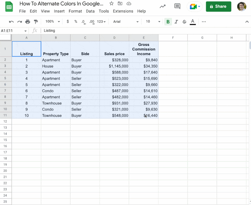
For this guide, i’ll choose the range a1:h20. Open the format menu and select the alternating colors option near the bottom. Before you add alternating rows to your spreadsheet, you need to first select the cells you want to apply this appearance to. Here’s how to alternate colors in google sheets: Got to format > alternating colors;

How to Format and Apply Alternating Colors in Google Sheets

This will apply a basic alternate color scheme to each row of your data set and. Converting a table to a range in google sheets. Web visit the google sheets website, sign in, and open the sheet where you want to apply alternating colors. Select the cells you want to color code. You can, however, add different colors to specific.

How to Alternate Row or Column Shading in Google Sheets

With the data selected, click on the format menu to open up various formatting options. Web visit the google sheets website, sign in, and open the sheet where you want to apply alternating colors. Click “format” > “conditional formatting.” choose “custom formula is” and enter =mod (row (),2)=0 for even rows. Web start by selecting the range of columns you.

How To Alternate Colors In Google Sheets For Rows And Columns

Click and drag to select the range of cells you want to format. Click done to apply the selected style to the range. While doing so, make sure to add the headers as well in this selection. Select “alternating colors” from the dropdown menu. If you only want to color the rows, don’t worry about selecting the entire column;

How to Alternate Colors in Google Sheets

You can, however, add different colors to specific cells afterwards. Click on the “format” tab in the menu bar. Web start by selecting the range of columns you want to format, navigate to the “format” menu, and choose “alternating color.”. Web hover over “alternating colors” and select your preferred color scheme from the provided options. Web to alternate row color.

How to use alternate colors in Google Sheets Paper Writer

When the cells are selected, click on the format tab from the top toolbar and select alternating colors. Web first, open the sheet and select the data range in which you’d want to color alternate rows. Here’s how to alternate colors in google sheets: Add alternating colors to rows. Web to do so, open your google sheets spreadsheet and select.

How to Alternate Row Colors in Google Sheets LiveFlow

This can be a group of. Web visit the google sheets website, sign in, and open the sheet where you want to apply alternating colors. When selecting the range, make sure to include all the rows and columns that you want to format. You can't do that using… Select one of the default styles and click done:

How to Alternate Row Colors in Google Sheets YouTube

This can be a column, row, or even the entire dataset. Web learn how to alternate colors by row or column in google sheets within a data table. Click and drag to select the range of cells you want to format. Choose from the default styles available. Got to format > alternating colors;

How To Format And Apply Alternating Colors In Google Sheets groovypost

Using alternate colors in google sheets will make your spreadsheets look more professional and easier to read. Web select all the rows you want to add the alternate colors. To convert a table back to a range, follow these steps: You can, however, add different colors to specific cells afterwards. Web visit the google sheets website, sign in, and open.

How To Alternate Colors In Google Sheets - Web how to color alternate rows in google sheets. Choose your desired colors for the even and odd rows by clicking on the color swatches. Select the range of cells you wish to apply the alternating colors to. This can be a group of. Simply open the menu and click format > alternating colors. However, you can customize the shade color and intensity to your preference. As you can see, it is a straightforward process. Open a web browser on your computer and head over to the google sheets website. After your data is selected, click format > alternating colors. Select the cells you want to color code.

Web alternate row colors in google sheets. This will open the ‘ alternating colors ’ toolbar on the right. Select the cells you want to apply the color scheme to; Web from the dropdown menu that appears, hover over “alternating colors” and click on “add alternating colors.” google sheets will automatically apply a default shading color to the selected range. Select “alternating colors” from the dropdown menu.

Click “format” > “conditional formatting.” choose “custom formula is” and enter =mod (row (),2)=0 for even rows. Want to change the background color of every other row of your spreadsheet? Click and drag your mouse over the cells you want to apply the alternating colors to. When selecting the range, make sure to include all the rows and columns that you want to format.

Select a color scheme or theme and you're done! You can either do this manually or select a cell in your data set, and then press ctrl+a to select the data automatically. Web from the dropdown menu that appears, hover over “alternating colors” and click on “add alternating colors.” google sheets will automatically apply a default shading color to the selected range.

If your sheet has a header or footer, you should include it in your selection, as well. This can be a group of. Using alternate colors in google sheets will make your spreadsheets look more professional and easier to read.

Click And Drag Your Mouse Over The Cells You Want To Apply The Alternating Colors To.

Before you add alternating rows to your spreadsheet, you need to first select the cells you want to apply this appearance to. Google sheets will automatically apply the chosen color scheme to the selected rows, alternating the colors between each row. Web first, open the sheet and select the data range in which you’d want to color alternate rows. In the sidebar that opens, uncheck the header checkbox to format the range as alternating colors, then select a style from the list of default styles.

We'll Start With Basics Where We Change The Color For Every Other Row, Then Move To 2 Or More.

Web start by selecting the range of columns you want to format, navigate to the “format” menu, and choose “alternating color.”. Web this new sheets feature has been around for many years in excel and has recently reached google. While doing so, make sure to add the headers as well in this selection. Click “format” > “conditional formatting.” choose “custom formula is” and enter =mod (row (),2)=0 for even rows.

Select The Range You Want To Apply Alternating Colors To.

Once you have logged in, create a new spreadsheet by clicking on “blank” in the “start a new spreadsheet” section. Google sheets will automatically apply the color scheme to the selected columns. Choose from the default styles available. This can be a column, row, or even the entire dataset.

Click On The Alternating Colors Option.

Converting a table to a range in google sheets. Web google sheets will add field labels in the top row like “column 1”, “column 2”,. Select the range of cells you want to format. You can either do this manually or select a cell in your data set, and then press ctrl+a to select the data automatically.